Today, we are delighted to announce PyTorch/XLA SPMD: the integration of GSPMD into PyTorch with an easy to use API. PyTorch developers seeking superior performance and scale can train and serve the largest neural networks while maximizing utilization of AI accelerators, such as Google Cloud TPUs.
Introduction
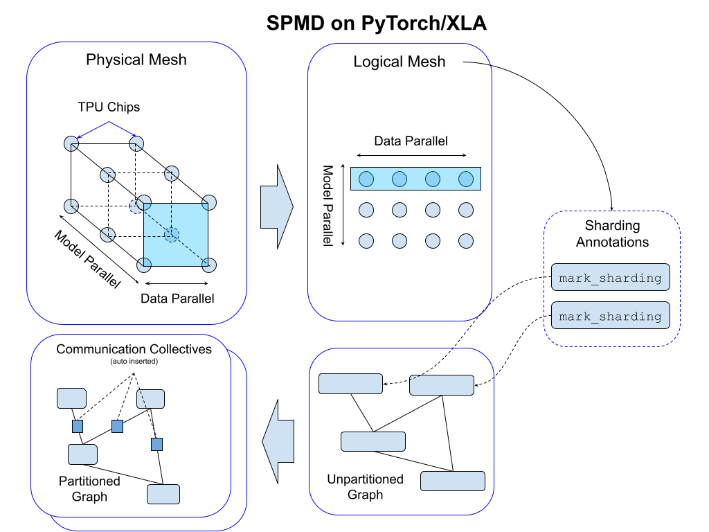
GSPMD is an automatic parallelization system for ML workloads. The XLA compiler transforms the single device program into a partitioned one with proper collectives, based on the user provided sharding hints. This allows developers to write PyTorch programs as if they are on a single large device without any custom sharded computation and/or collective communication ops to scale models.
PyTorch/XLA SPMD allows PyTorch users to parallelize their ML workloads with GSPMD with less effort and with better performance. Some of the key highlights are:
- Better developer experience. Everything happens with a few sharding annotations from the user, and PyTorch/XLA SPMD achieves comparable performance to the most efficient PyTorch sharding implementation (see the Examples and Results section below). PyTorch/XLA SPMD separates the task of programming an ML model from the challenge of parallelization. Its automated approach to model sharding frees up the user from implementing the sharded version of ops with proper collectives in place.
- A single API that enables a large variety of parallelism algorithms (including data parallelism, fully sharded data parallelism, spatial partitioning tensor and pipeline parallelism, as well as combinations of these algorithms) for different ML workloads and model architectures.
- Industry-leading performance in large model training. PyTorch/XLA SPMD brings the powerful XLA GSPMD to PyTorch, enabling users to harness the full power of Google Cloud TPUs.
- Enabling PyTorch and JAX developers take advantage of the same underlying XLA API to scale models.
Key Concepts
The key concepts behind the sharding annotation API are: 1) Mesh, 2) Partition Spec, and 3) mark_sharding API to express sharding intent using Mesh and Partition Spec. A more detailed design overview is available as a user guide here.
Mesh
For a given cluster of devices, a physical mesh is a representation of the interconnect topology.
We derive a logical mesh based on this topology to create sub-groups of devices which can be used for partitioning different axes of tensors in a model. We apply sharding annotations to map the program across the logical mesh; this automatically inserts communication collectives in the program graph to support functional correctness (see the figure below).

We abstract logical mesh with Mesh API. The axes of the logical Mesh can be named. Here is an example:
import numpy as np
import torch_xla.runtime as xr
import torch_xla.experimental.xla_sharding as xs
from torch_xla.experimental.xla_sharding import Mesh

# Enable XLA SPMD execution mode.
xr.use_spmd()

# Assuming you are running on a TPU host that has 8 devices attached
num_devices = xr.global_runtime_device_count()
# mesh shape will be (4,2) in this example
mesh_shape = (num_devices // 2, 2)
device_ids = np.array(range(num_devices))
# axis_names 'x' nad 'y' are optional
mesh = Mesh(device_ids, mesh_shape, ('x', 'y'))

mesh.get_logical_mesh()
>> array([[0, 1],
          [2, 3],
          [4, 5],
          [6, 7]])
mesh.shape()
>> OrderedDict([('x', 4), ('y', 2)])
Partition Spec
partition_spec has the same rank as the input tensor. Each dimension describes how the corresponding input tensor dimension is sharded across the device mesh (logically defined by mesh_shape). partition_spec is a tuple of device_mesh dimension index, None, or a tuple of mesh dimension indices. The index can be an int or str if the corresponding mesh dimension is named. This specifies how each input rank is sharded (index to mesh_shape) or replicated (None).
# Provide optional mesh axis names and use them in the partition spec
mesh = Mesh(device_ids, (4, 2), ('data', 'model'))
partition_spec = ('model', 'data')
xs.mark_sharding(input_tensor, mesh, partition_spec)
We support all three types of sharding described in the original GSPMD paper. For instance, one can specify partial replication like this:
# Provide optional mesh axis names and use them in the partition spec
mesh = Mesh(device_ids, (2, 2, 2), ('x', 'y', 'z'))

# evenly shard across x and z and replicate among y
partition_spec = ('x', 'z')  # equivalent to ('x', None, 'z')
xs.mark_sharding(input_tensor, mesh, partition_spec)
Simple Example With Sharding Annotation
Users can annotate native PyTorch tensors using the mark_sharding API (src). This takes torch.Tensor as input and returns a XLAShardedTensor as output.
def mark_sharding(t: Union[torch.Tensor, XLAShardedTensor], mesh: Mesh, partition_spec: Tuple[Union[int, None]]) -> XLAShardedTensor
Invoking mark_sharding API takes a user defined logical mesh and partition_spec and generates a sharding annotation for the XLA compiler. The sharding specification is attached to the XLATensor, as well as the original input tensor. Here is a simple usage example from the [RFC], to illustrate how the sharding annotation API works:
import numpy as np
import torch
import torch_xla.core.xla_model as xm
import torch_xla.runtime as xr
import torch_xla.experimental.xla_sharding as xs
from torch_xla.experimental.xla_sharded_tensor import XLAShardedTensor
from torch_xla.experimental.xla_sharding import Mesh

# Enable XLA SPMD execution mode.
xr.use_spmd()

# Device mesh, this and partition spec as well as the input tensor shape define the individual shard shape.
num_devices = xr.global_runtime_device_count()
mesh_shape = (2, num_devicese // 2)  # 2x4 on v3-8, 2x2 on v4-8
device_ids = np.array(range(num_devices))
mesh = Mesh(device_ids, mesh_shape, ('x', 'y'))

t = torch.randn(8, 4).to(xm.xla_device())

# Mesh partitioning, each device holds 1/8-th of the input
partition_spec = (0, 1)
m1_sharded = xs.mark_sharding(t, mesh, partition_spec)
assert isinstance(m1_sharded, XLAShardedTensor) == True
# Note that the sharding annotation is also in-placed updated to t
We can annotate different tensors in the PyTorch program to enable different parallelism techniques, as described in the comment below:
# Sharding annotate the linear layer weights. SimpleLinear() is a nn.Module.
model = SimpleLinear().to(xm.xla_device())
xs.mark_sharding(model.fc1.weight, mesh, partition_spec)

# Training loop
model.train()
for step, (data, target) in enumerate(loader):
  # Assumes `loader` returns data, target on XLA device
  optimizer.zero_grad()
  # Sharding annotate input data, we can shard any input
  # dimensions. Sharding the batch dimension enables
  # data parallelism, sharding the feature dimension enables
  # spatial partitioning.
  xs.mark_sharding(data, mesh, partition_spec)
  ouput = model(data)
  loss = loss_fn(output, target)
  optimizer.step()
  xm.mark_step()
More complete unit test cases and integration test examples are available in the PyTorch/XLA repo.
Results
Performance
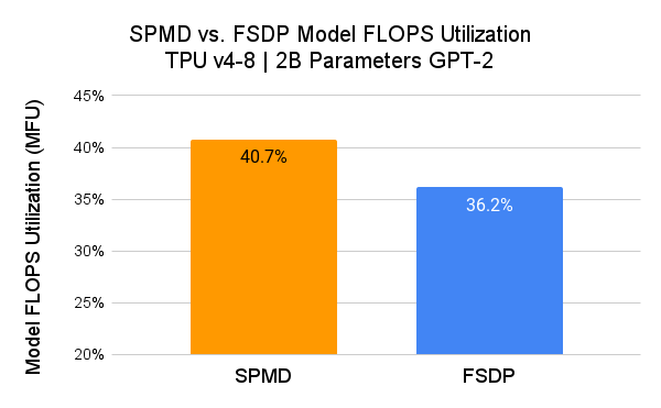
We measured the performance of PyTorch/XLA SPMD using a GPT-2 model (src) and compared it with user-mode FSDP.
Here, SPMD applies the same sharding scheme as the FSDP plot (i.e. 1D sharding). Users are expected to achieve better MFU results by exploring more advanced SPMD sharding schemes.

We use Model FLOPS Utilization (MFU) as a metric for comparison. MFU is “the ratio of the observed throughput relative to the theoretical maximum throughput of a system operating at peak FLOPs” (PaLM paper).
flops_per_step = 6 * global_batch_size * seq_len * num_params
model_flops_utilization = flops_per_step / step_time(s) / chip_count / flops_per_chip
This estimation assumes that the input dimensionality is much larger than the input sequence length (d_model » seq_len). If this assumption is violated the self-attention FLOPs start to be significant enough and this expression will underestimate the true MFU.
Scalability
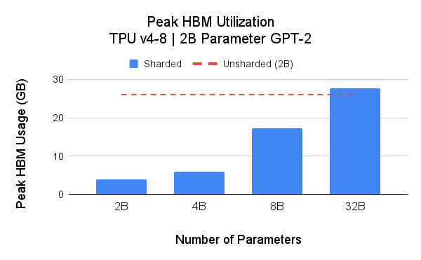
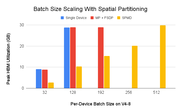
One of the core benefits of SPMD is the flexible partitioning which can be used to save accelerator memory (HBM) usage and improve scalability. For scalability analysis, we present two studies: 1) we examine the peak HBM across 4 model sizes using Hugging Face transformers (GPT-2) as the base implementation; 2) we examine the peak HBM usage with spatial partitioning.

The above figure illustrates the unsharded 2B parameters model peak memory footprint stands at 26GB (red dashed line). harding model weights (model parallelism) reduces the peak memory footprint, and thus, enables larger model training with a given TPU pod slice. In these experiments, we achieved up to 39.75% MFU on a 4B parameters model on Google Cloud TPU v4-16.
We also ran an input batch scalability test using spatial partitioning and a simple ResNet50 example (src) on Cloud TPU v4-8. Input batch is commonly sharded across the batch dimension for data parallelism (DDP, FSDP), but PyTorch/XLA SPMD enables input sharding across input feature dimensions for spatial sharding. As shown in the below figure, one can push the per-device batch size to 512 with spatial partitioning which is not possible with other data parallelism techniques.

The Road Forward for PyTorch/XLA SPMD
We are ecstatic about what’s ahead for PyTorch/XLA and invite the community to join us. SPMD is still experimental, and we continuously add new features to it. In future releases, we plan to address async dataloading, partially replicated sharding, and other improvements. We’d love to hear from you, answer your questions about PyTorch/XLA SPMD, and learn how you use SPMD.
Cheers!
The PyTorch/XLA Team at Google
